[1]:
import numpy as np
import psdr, psdr.demos
import matplotlib.pyplot as plt
import matplotlib.patches as mpatches
%matplotlib inline
%config InlineBackend.figure_format = 'retina'
Assessing Smoothness
Most parameter space dimension reduction techniques make a tacit assumption that the function we are working with is at least Lipschitz continuous. There is a simple reason: if we cannot assume some degree of regularity for the function, then dimension reduction becomes untractible. Hence it is important to check if the model we have constructed is continuous with respect to its inputs. One way to check for smoothness is to perform a “parameter sweep.” Given a point in the domain,
\(\mathbf{x}\in \mathcal{D}\), we draw a line in the direction \(\mathbf{p}\) extending in either direction to the boundary of the domain. The function domain.sweep provides a helper for doing so. We then check for smoothness by plotting the value of \(f(\mathbf{x})\) along this line.
[2]:
dom = psdr.BoxDomain([-1,-1], [1,1])
x = [0.5, 0]
p = [0.5, 0.5]
X, y = dom.sweep(x = x, p = p)
fun = psdr.Function(lambda x: x[0]*x[1], dom)
# Draw the sweep
fig, axes = plt.subplots(1,2, figsize = (10,5))

ax = axes[0]
rect = mpatches.Rectangle([-1,-1], 2, 2, ec="none", fc = 'black', alpha = 0.1)
ax.add_patch(rect)
ax.plot(X[:,0], X[:,1], 'k.-', markersize = 10) # points on the sweep
ax.plot(x[0], x[1], 'ro') # The point the sweep passes through
ax.axis('equal')
ax.set_title('Sweep Locations')
ax.axis('off');

ax = axes[1]
fX = fun(X)
ax.plot(y, fX, 'k.')
ax.set_ylabel('$f(\mathbf{x})$')
ax.set_xlabel('length along sweep')
ax.set_title('Function along the sweep')
fig.tight_layout();
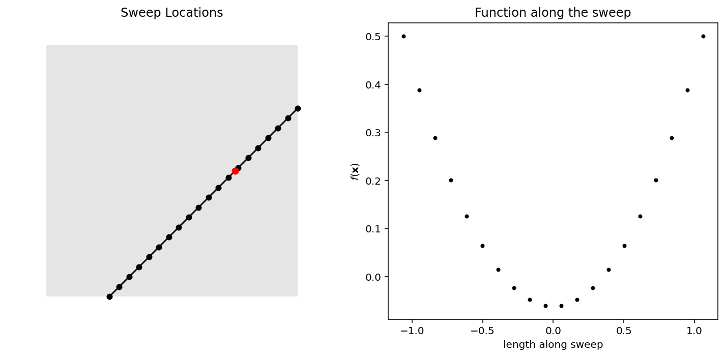
In this artifical example above, we see that the quadratic function \(f(\mathbf{x}) = x_1x_2\) is indeed smooth.
Non-smooth functions
However, with complex simulations this need not be the case. In the following example we consider the NACA0012 airfoil design problem where enlarged the domain and decreased the number of iterations such that discontinuities appear.
[3]:
# Cache the data to reduce running time
try:
    X = np.loadtxt('data/sweep_naca_X.dat')
    fX = np.loadtxt('data/sweep_naca_10_fX.dat')
    d = (X[1] - X[0])/np.linalg.norm(X[1] - X[0])
    y = X.dot(d)
except:
    fun = psdr.demos.NACA0012(maxiter = 10, verbose = False, fraction = 0.1)
    x = np.zeros(len(fun.domain))
    p = np.ones(len(fun.domain))
    X, y = fun.domain.sweep(n = 20, x = x, p = p)
    fX = fun(X)
    np.savetxt('data/sweep_naca_X.dat', X)
    np.savetxt('data/sweep_naca_10_fX.dat', fX)
[4]:
fig, axes = plt.subplots(1,2, figsize = (10,5))
axes[0].plot(y, fX[:,0], '.')
axes[0].set_title('Lift')
axes[1].plot(y, fX[:,1], '.')
axes[1].set_title('Drag')
for ax in axes:
    ax.set_xlabel('length along sweep')
    ax.set_ylabel('$f(\mathbf{x})$')
fig.tight_layout()
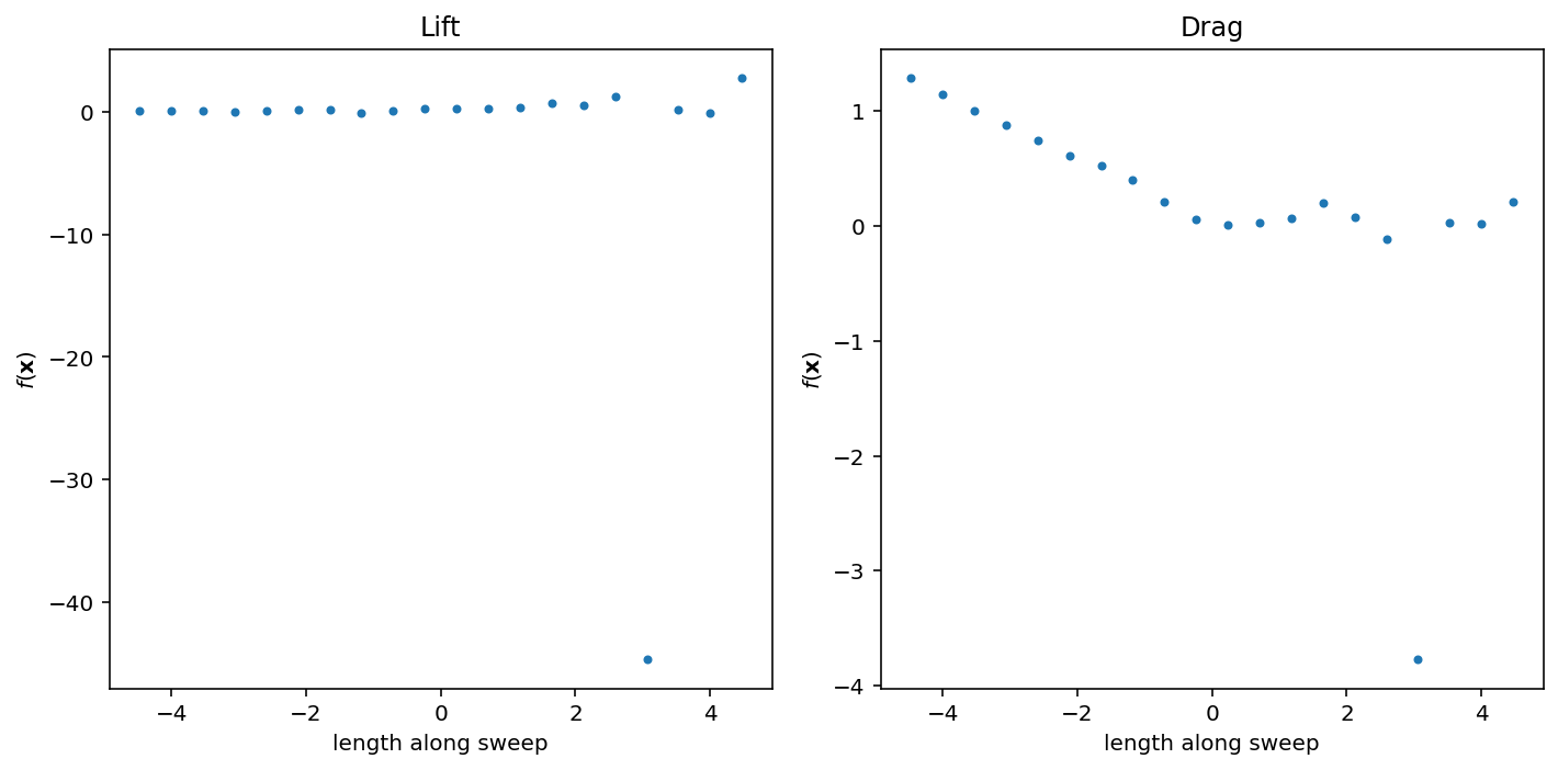
Here we see a jump discontinuity on the right side of each plot.
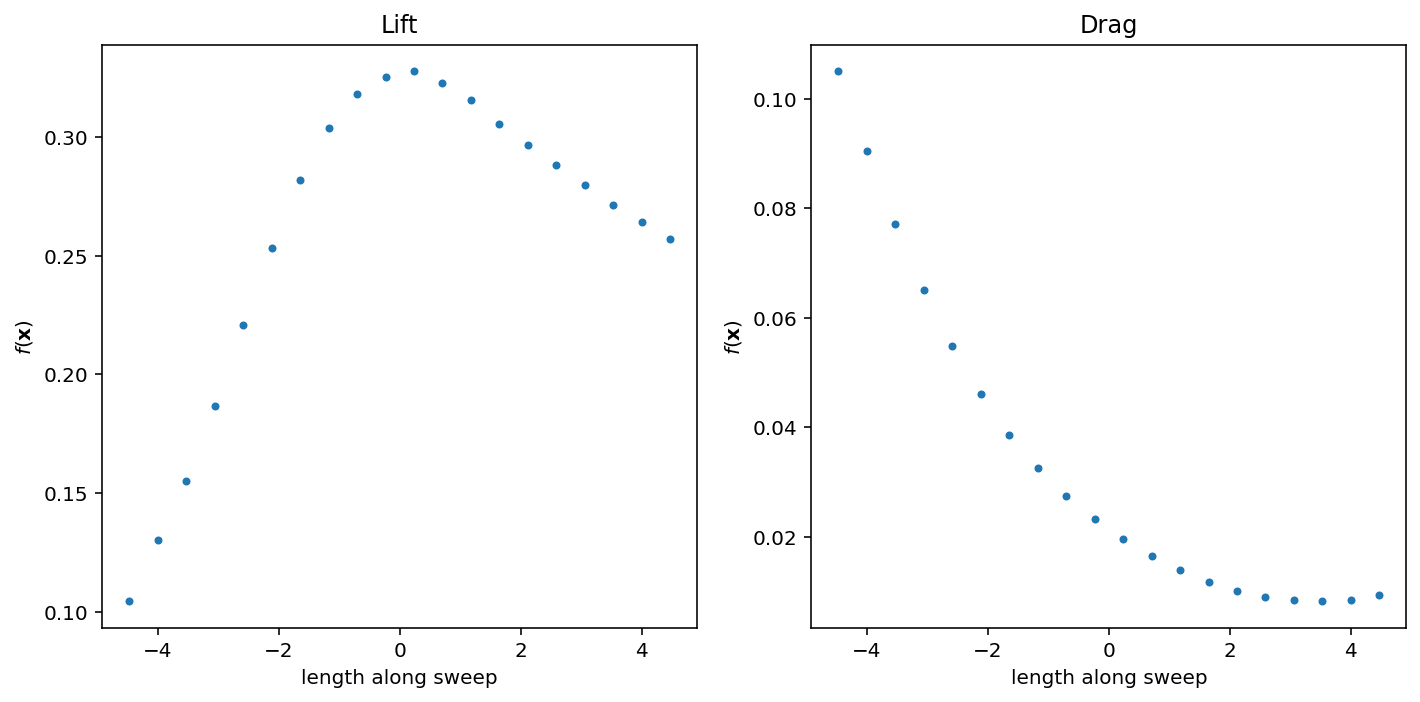
However, if we shrink the domain and use more iterations (back to the defaults) we observe a smooth function.
[5]:
# Cache the data to reduce running time
try:
    X = np.loadtxt('data/sweep_naca_X.dat')
    fX = np.loadtxt('data/sweep_naca_1000_fX.dat')
    d = (X[1] - X[0])/np.linalg.norm(X[1] - X[0])
    y = X.dot(d)
except:
    fun = psdr.demos.NACA0012(maxiter = 1000, verbose = False, fraction = 0.01)
    X = np.loadtxt('data/sweep_naca_X.dat')
    fX = fun(X)
    np.savetxt('data/sweep_naca_1000_fX.dat', fX)
[6]:
fig, axes = plt.subplots(1,2, figsize = (10,5))
axes[0].plot(y, fX[:,0], '.')
axes[0].set_title('Lift')
axes[1].plot(y, fX[:,1], '.')
axes[1].set_title('Drag')
for ax in axes:
    ax.set_xlabel('length along sweep')
    ax.set_ylabel('$f(\mathbf{x})$')
fig.tight_layout()
[ ]: